Bookstore vs Income Part 7

See here for part1, part2, part3 part4, part5, part 6

Now know how to annotate the data points, I can now annotate the outliers which I originally wanted to.

Looking back at the database of income I noticed that some of the data points have the wrong incomes. I started to check this because the “city of Westminster” data point had a low income for its location. I think this error happed because in the count_borough csv I had “Westminster” as “City of Westminster” changing the order of the dataset. So, when the Incomes were added the Croydon income (next data point after the city of Westminster) was added to the Westminster data point.

Name of Westminster data point in income excel file

Name of Westminster data point in my count of bookstores in the borough.

I worked on adjusting the count dataset. Using pandas to converting it into a dataframe, adding column names. And removing the 'London Borough of’ and ‘'Royal Borough of’ prefixes. The stuff I did manually first time round.

bookstore_df = pd.read_csv('filtered_dataset_boroughs.csv')
count = bookstore_df['Borough'].value_counts().rename_axis('Borough').reset_index(name='Count')
print(count)

count['Borough'] = count['Borough'].str.replace('London Borough of ', '')
count['Borough'] = count['Borough'].str.replace('Royal Borough of ', '')
count['Borough'] = count['Borough'].str.replace('City of Westminster ', 'Westminster')

print(count)

Next I compared the names of the count dataframe and the income names. To find the missing values after value count. As the value count does not return any values that did not occur once.

compare_1 = tax_year_without_pop['Area'].reset_index(drop=True)
compare_2 = count['Borough']
compare_1 = compare_1.sort_values()
compare_2 = compare_2.sort_values().reset_index(drop=True)
# print(compare_1)
# print(compare_2)

idx1 = pd.Index(compare_1)
idx2 = pd.Index(compare_2)
print(idx1.difference(idx2).values)
append_values = idx1.difference(idx2).values

['Barking and Dagenham' 'Bexley' 'Brent' 'City of London' 'Hackney'
 'Hammersmith and Fulham' 'Kingston-upon-Thames' 'Lambeth' 'Newham'
 'Richmond-upon-Thames' 'Southwark' 'Westminster']

A few are duplicates but they can be removed after adding to the dataframe. To add to dataframe I need to turn this list into the dataframe as the same shape as the one I wanted to append to.

First I made a list a zeros with same length as the list.

zero_list = [0] * len(append_values)
[0, 0, 0, 0, 0, 0, 0, 0, 0, 0, 0, 0]

Made a new dataframe object by zipping the list up:

extra_name_df = pd.DataFrame(list(zip(append_values, zero_list)), columns=['Borough', 'Count'])

Now I need to get rid of the duplicates like Richmond, Kingston and Westminster.

extra_name_df = extra_name_df.drop([3, 6, 9, 11])

Then appended this dataframe with my exiting dataframe.

count = count.append(extra_name_df, ignore_index=True)

Now I can update the count_borough CSV file used to plot the data.

count.to_csv('count_borough.csv').

I later had to just the code above due some values being missing and the Westminster still having the city word changing the order of the dataset.

Next is to add the general direction of the borough. Using compass names like last time. The Boroughs were reorganised using this Wikipedia page. A government plan on how is London is split into sub-regions.

Using the table, I converted the value into a regex pattern so pandas can scan strings in my dataframe and return the sub-region.

North_names = '(Barnet|Enfield|Haringey)'
South_names = '(Bromley|Croydon|Kingston upon Thames|Merton|Sutton|Wandsworth)'
East_names = '(Barking and Dagenham|Bexley|Greenwich|Hackney|Havering|Lewisham|Newham|Redbridge|Tower Hamlets|Waltham Forest)'
West_names = '(Brent|Ealing|Hammersmith and Fulham|Harrow|Richmond upon Thames|Hillingdon|Hounslow)'
Central_names = '(Camden|City of London|Kensington and Chelsea|Islington|Lambeth|Southwark|Westminster)'

Then created a new column with the same length borough column. Where the sub-regions will be stored. count_df['Compass'] = [0] * len(count_df['Borough']) I used Boolean masking to return a string if pandas contains function matches true.

count_df['Compass'] = count_df['Compass'].mask((count_df['Borough'].str.contains(
    North_names) == True), other='North')

count_df['Compass'] = count_df['Compass'].mask((count_df['Borough'].str.contains(
    South_names) == True), other='South')

count_df['Compass'] = count_df['Compass'].mask((count_df['Borough'].str.contains(
    East_names) == True), other='East')

count_df['Compass'] = count_df['Compass'].mask((count_df['Borough'].str.contains(
    West_names) == True), other='West')

count_df['Compass'] = count_df['Compass'].mask((count_df['Borough'].str.contains(
    Central_names) == True), other='Central')

Now I can update the CSV file which saves this dataframe.

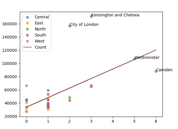
count_df.to_csv('Borough_income_count.csv', index=False)

Now running the previous matplotlib code I get this result:

As we can see the values have changed quite a bit. Croydon is label because in the last graph the index was the value of the city of Westminster. I will now adjust the annotation so it can annotate Westminster, not Croydon.

I also added the line show the correlation in the graph

x = compass_df['Count'].astype('float')
y = compass_df['Income'].astype('float')

b, m = polyfit(x, y, 1)
plt.plot(x, b + m * x, '-')

I later changed the transparency of the data point increase the look of the graph.

for name, group in groups:
    ax.plot(group["Count"], group["Income"], marker="o", linestyle="", label=name, alpha=0.6)